If recently we used best subset as a way of reducing the unnecessary model complexity, this time we are going to use the Ridge regression technique.

Both the lasso and ridge regression are called shrinkage methods. The best subset method uses least squares to fit a model with a subset of predictors. Alternatively, shrinkage methods use all predictors but constraining and regularising them towards zero. One major difference between them, is that ridge will end up using all the predictors, while the lasso shrink some of them up to the point of making them zero.

Again we will use the classic swiss data set provided with R datasets.

data(swiss)
?swiss

And again we are interested in predicting infant mortality of an hypotetical commune using a multi-linear model. In the previous post we could see a quick exploratory analysis of the correlation between the different variables.

The glmnet package provides methods to perform ridge regression and the lasso. The main function in the package is glmnet(). This function has a different syntax from other model-fitting functions in R. This time we must pass in an x matrix as well as a y vector, and we do not use the familiar y ∼ x syntax.

x <- model.matrix(Infant.Mortality~., swiss)[,-1]
y <- swiss$Infant.Mortality

A quick look at the first rows of the matrix shows that basically contains values for the 5 predictors in each of the comunes.

head(x,5)

##              Fertility Agriculture Examination Education Catholic
## Courtelary        80.2        17.0          15        12     9.96
## Delemont          83.1        45.1           6         9    84.84
## Franches-Mnt      92.5        39.7           5         5    93.40
## Moutier           85.8        36.5          12         7    33.77
## Neuveville        76.9        43.5          17        15     5.16

The glmnet() function takes an alpha argument that determines what method is used. If alpha=0 then ridge regression is used, while if alpha=1 then the lasso is used. We will start with the former.

library(glmnet)
ridge.mod <- glmnet(x, y, alpha=0, nlambda=100, lambda.min.ratio=0.0001)

By default the glmnet function performs ridge regression for an automatically selected range of λ values (the shrinkage coefficient). The values are based on nlambda and lambda.min.ratio. Associated with each value of λ is a vector of regression coefficients. For example, the 100th value of λ, a very small one, is closer to perform least squares:

ridge.mod$lambda[100]

## [1] 0.12

coef(ridge.mod)[,100]

## (Intercept)   Fertility Agriculture Examination   Education    Catholic 
##   10.266651    0.133406   -0.015177    0.032356    0.042854    0.002024

While the 1st one is the null model containing just the intercept, due to the shrinkage of all the predictor coefficients:

ridge.mod$lambda[1]

## [1] 1200

coef(ridge.mod)[,1]

## (Intercept)   Fertility Agriculture Examination   Education    Catholic 
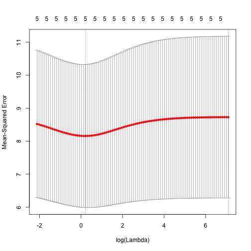
##   1.994e+01   9.811e-38  -7.884e-39  -4.205e-38  -3.039e-38   1.238e-38

But it would be better to use cross-validation to choose λ. We can do this using cv.glmnet. By default, the function performs ten-fold cross-validation:

set.seed(1)
cv.out <- cv.glmnet(x, y, alpha=0, nlambda=100, lambda.min.ratio=0.0001)
plot(cv.out)

best.lambda <- cv.out$lambda.min
best.lambda

## [1] 1.229

Once we have the best lambda, we can use predict to obtain the coefficients.

predict(ridge.mod, s=best.lambda, type="coefficients")[1:6, ]

## (Intercept)   Fertility Agriculture Examination   Education    Catholic 
##   15.059642    0.075000   -0.015272    0.008441    0.006728    0.004445

Next time, the lasso.