Linear regression models are easy to fit and interpret. Moreover, they are suprisingly accurate in many real world situations where the relationship between the response and the predictors is approximately linear. However, it is often the case that not all the variables used in a multiple regression model are in associated with the response.

Including irrelevant variables leads to unnecessary complexity. By removing them we can obtain a model that is more easily interpreted. Additionally, when the number of predictors is close to the number of samples, linear models tend to overfit and therefore to perform badly in their further predictions.

The best subset model selection approach identifies a subset of the predictors that show to be related to the response. We can then fit a model using least squares on the reduced set of variables.

Here, we are going to do that using R.

The swiss data set

We will use the classic swiss data set provided with R datasets. We can have a look at its documentation.

data(swiss)
?swiss

There we see that contains standardized fertility measure and socio-econimic indicators for each of the 47 French-speaking provinces of Switzerlad at about 1888. It is composed by 47 observations on 6 variables, each of which is in percent (i.e. in [0, 100]), including:

• Fertility.
• Agriculture in % of men involded in agriculture as occupation.
• Examination as % draftees receiving highest mark on army examination.
• Education as % of education beyond primary school for draftees.
• Catholic as % of catholic (as opposed to protestant).
• Infant mortality as % of live births who live less than 1 year.

We are interested in predicting infant mortality using a multi-linear model.

We can have a quick look at how these variables interact using some plts.

pairs(swiss)

And the correlation matrix.

cor(swiss)

##                  Fertility Agriculture Examination Education Catholic
## Fertility           1.0000     0.35308     -0.6459  -0.66379   0.4637
## Agriculture         0.3531     1.00000     -0.6865  -0.63952   0.4011
## Examination        -0.6459    -0.68654      1.0000   0.69842  -0.5727
## Education          -0.6638    -0.63952      0.6984   1.00000  -0.1539
## Catholic            0.4637     0.40110     -0.5727  -0.15386   1.0000
## Infant.Mortality    0.4166    -0.06086     -0.1140  -0.09932   0.1755
##                  Infant.Mortality
## Fertility                 0.41656
## Agriculture              -0.06086
## Examination              -0.11402
## Education                -0.09932
## Catholic                  0.17550
## Infant.Mortality          1.00000

We can see that Infant.Mortality is positively correlated with Fertility (obviously) with being Catholic and negatively with Examination and Education. Additionally we see that Fertility is positively correlated with being Catholic and with Agriculture and negatively with Edication and Examination.

Let us now select among these predictors using best subset selection. The function regsubsets in the leaps package does exactly this. It performs best predictor subset selection by identifying the best model that contains a given number of predictors, where best is quantified using RSS.

The summary() command outputs the best set of variables for each model size.

library(leaps)
best.subset <- regsubsets(Infant.Mortality~., swiss, nvmax=5)
best.subset.summary <- summary(best.subset)
best.subset.summary$outmat

##          Fertility Agriculture Examination Education Catholic
## 1  ( 1 ) "*"       " "         " "         " "       " "     
## 2  ( 1 ) "*"       " "         " "         "*"       " "     
## 3  ( 1 ) "*"       "*"         " "         "*"       " "     
## 4  ( 1 ) "*"       "*"         "*"         "*"       " "     
## 5  ( 1 ) "*"       "*"         "*"         "*"       "*"

The outmat field on the summary contains a matrix with the best subset of predictors for 1 to 5 predictor models. For example, the best model with two variables includes Fertility and Education as predictors for Infant.Mortality. We can also see that all models include Fertility, and that all models with at least two variables include also Education. The summary object also includes metrics such as adjusted R2, CP, or BIC, that we can use to determine the best overall model.

best.subset.by.adjr2 <- which.max(best.subset.summary$adjr2)
best.subset.by.adjr2

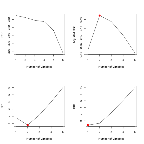
## [1] 2

Adjusted R2 tells us that the best model is that with two variables, that is Fertility and Education.

best.subset.by.cp <- which.min(best.subset.summary$cp)
best.subset.by.cp

## [1] 2

Using CP we arrive to the same conclusion.

best.subset.by.bic <- which.min(best.subset.summary$bic)
best.subset.by.bic

## [1] 1

However using BIC we should go for the model using just Fertility as a predictor. We can plot this information.

par(mfrow=c(2,2))
plot(best.subset$rss, xlab="Number of Variables", ylab="RSS", type="l")
plot(best.subset.summary$adjr2, xlab="Number of Variables", ylab="Adjusted RSq", type="l")
points(best.subset.by.adjr2, best.subset.summary$adjr2[best.subset.by.adjr2], col="red", cex =2, pch =20)
plot(best.subset.summary$cp, xlab="Number of Variables", ylab="CP", type="l")
points(best.subset.by.cp, best.subset.summary$cp[best.subset.by.cp], col="red", cex =2, pch =20)
plot(best.subset.summary$bic, xlab="Number of Variables", ylab="BIC", type="l")
points(best.subset.by.bic, best.subset.summary$bic[best.subset.by.bic], col="red", cex =2, pch =20)

From there we can see that the 2-variable model is not that bad regarding the BIC coefficient. So, as a conclusion, we show the coefficients of the 2-variable model using Fertility and Education as inputs to predict Infant.Mortality.

coef(best.subset,2)

## (Intercept)   Fertility   Education 
##     8.63758     0.14615     0.09595